HPMC User Guide v 1.00
© 2022 Bassem W. Jamaleddine
The HPMC computer has a GPU that allows you to run CUDA related programs. Your HPMC has been already configured with the essential device drivers so that the GPU can serve you to run any of the following: torch, pytorch, theano, caffe, cuda, and pycuda.
■ About your HPMC CUDA Device
# checkDeviceInfor
20:00 root@HPMC7: /appz/professional-c-cuda-programming/CodeSamples/chapter02 #  ./checkDeviceInfor
./checkDeviceInfor Starting...
Detected 1 CUDA Capable device(s)
Device 0: "GeForce GTX TITAN X"
  CUDA Driver Version / Runtime Version          9.2 / 6.5
  CUDA Capability Major/Minor version number:    5.2
  Total amount of global memory:                 11.93 MBytes (12805668864 bytes)
  GPU Clock rate:                                1240 MHz (1.24 GHz)
  Memory Clock rate:                             3505 Mhz
  Memory Bus Width:                              384-bit
  L2 Cache Size:                                 3145728 bytes
  Max Texture Dimension Size (x,y,z)             1D=(65536), 2D=(65536,65536), 3D=(4096,4096,4096)
  Max Layered Texture Size (dim) x layers        1D=(16384) x 2048, 2D=(16384,16384) x 2048
  Total amount of constant memory:               65536 bytes
  Total amount of shared memory per block:       49152 bytes
  Total number of registers available per block: 65536
  Warp size:                                     32
  Maximum number of threads per multiprocessor:  2048
  Maximum number of threads per block:           1024
  Maximum sizes of each dimension of a block:    1024 x 1024 x 64
  Maximum sizes of each dimension of a grid:     2147483647 x 65535 x 65535
  Maximum memory pitch:                          2147483647 bytes
# ./simpleDeviceQuery
19:59 root@HPMC7: /appz/professional-c-cuda-programming/CodeSamples/chapter03 #  ./simpleDeviceQuery
Device 0: GeForce GTX TITAN X
  Number of multiprocessors:                     24
  Total amount of constant memory:               64.00 KB
  Total amount of shared memory per block:       48.00 KB
  Total number of registers available per block: 65536
  Warp size:                                     32
  Maximum number of threads per block:           1024
  Maximum number of threads per multiprocessor:  2048
  Maximum number of warps per multiprocessor:    64
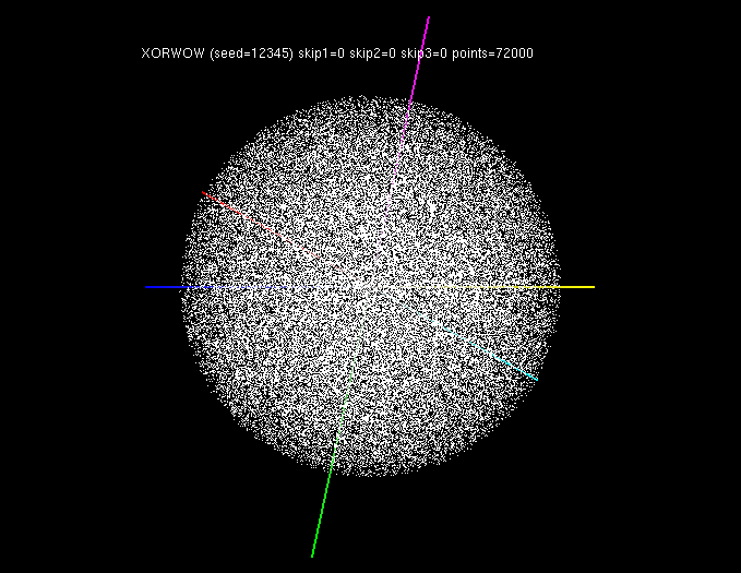
To make sure that your GPU is ready to serve CUDA programming capability, just invoke the randomFog program at the prompt. Figure shows the randomFog. In case the randomFog failed to execute then refer to Appendix Troubleshooting the CUDA GPU.
■ CUDNN with Torch
You program in Lua and run torch programs on your HPMC.torch: A Tensor library like NumPy, with strong GPU support PyTorch is used either as a replacement for NumPy to use the GPU as a processing agent. It is also used a platform for deep learning research.
# 20:09 root@HPMC7: /appz/torch # th bench.lua
20:09 root@HPMC7: /appz/torch #  th bench.lua
Found Environment variable CUDNN_PATH = /usr/local/cuda-9.2/lib64/libcudnn.so.7.1.4
Running on device: GeForce GTX TITAN X

CONFIG: input = 3x128x128 * ker = 3x96x11x11 (bs = 128, stride = 1)
cudnn.SpatialConvolution                :updateOutput():      51.10
cudnn.SpatialConvolution             :updateGradInput():      57.34
cudnn.SpatialConvolution           :accGradParameters():      50.86
cudnn.SpatialConvolution                         :TOTAL:     159.30
nn.SpatialConvolutionMM                 :updateOutput():      44.83
nn.SpatialConvolutionMM              :updateGradInput():      54.59
nn.SpatialConvolutionMM            :accGradParameters():      56.69
nn.SpatialConvolutionMM                          :TOTAL:     156.12
ccn2.SpatialConvolution                 :updateOutput():      32.38
ccn2.SpatialConvolution              :updateGradInput():      50.96
ccn2.SpatialConvolution            :accGradParameters():      44.72
ccn2.SpatialConvolution                          :TOTAL:     128.06

CONFIG: input = 64x64x64 * ker = 64x128x9x9 (bs = 128, stride = 1)
cudnn.SpatialConvolution                :updateOutput():      89.60
cudnn.SpatialConvolution             :updateGradInput():     264.64
cudnn.SpatialConvolution           :accGradParameters():     141.98
cudnn.SpatialConvolution                         :TOTAL:     496.21
nn.SpatialConvolutionMM                 :updateOutput():     138.05
nn.SpatialConvolutionMM              :updateGradInput():     219.20
nn.SpatialConvolutionMM            :accGradParameters():     330.22
nn.SpatialConvolutionMM                          :TOTAL:     687.47
ccn2.SpatialConvolution                 :updateOutput():     109.02
ccn2.SpatialConvolution              :updateGradInput():     125.64
ccn2.SpatialConvolution            :accGradParameters():     227.74
ccn2.SpatialConvolution                          :TOTAL:     462.40

CONFIG: input = 128x32x32 * ker = 128x128x9x9 (bs = 128, stride = 1)
cudnn.SpatialConvolution                :updateOutput():      30.75
cudnn.SpatialConvolution             :updateGradInput():      74.42
cudnn.SpatialConvolution           :accGradParameters():      54.36
cudnn.SpatialConvolution                         :TOTAL:     159.52
nn.SpatialConvolutionMM                 :updateOutput():      53.73
nn.SpatialConvolutionMM              :updateGradInput():     103.11
nn.SpatialConvolutionMM            :accGradParameters():      55.03
nn.SpatialConvolutionMM                          :TOTAL:     211.87
ccn2.SpatialConvolution                 :updateOutput():      37.26
ccn2.SpatialConvolution              :updateGradInput():      46.71
ccn2.SpatialConvolution            :accGradParameters():      85.09
ccn2.SpatialConvolution                          :TOTAL:     169.07

CONFIG: input = 128x16x16 * ker = 128x128x7x7 (bs = 128, stride = 1)
cudnn.SpatialConvolution                :updateOutput():       4.33
cudnn.SpatialConvolution             :updateGradInput():       7.33
cudnn.SpatialConvolution           :accGradParameters():       8.70
cudnn.SpatialConvolution                         :TOTAL:      20.36
nn.SpatialConvolutionMM                 :updateOutput():      14.75
nn.SpatialConvolutionMM              :updateGradInput():      18.78
nn.SpatialConvolutionMM            :accGradParameters():      12.61
nn.SpatialConvolutionMM                          :TOTAL:      46.14
ccn2.SpatialConvolution                 :updateOutput():       4.57
ccn2.SpatialConvolution              :updateGradInput():       4.29
ccn2.SpatialConvolution            :accGradParameters():       7.69
ccn2.SpatialConvolution                          :TOTAL:      16.55

CONFIG: input = 384x13x13 * ker = 384x384x3x3 (bs = 128, stride = 1)
cudnn.SpatialConvolution                :updateOutput():       7.77
cudnn.SpatialConvolution             :updateGradInput():      11.71
cudnn.SpatialConvolution           :accGradParameters():      12.91
cudnn.SpatialConvolution                         :TOTAL:      32.39
nn.SpatialConvolutionMM                 :updateOutput():      13.15
nn.SpatialConvolutionMM              :updateGradInput():      17.28
nn.SpatialConvolutionMM            :accGradParameters():      14.63
nn.SpatialConvolutionMM                          :TOTAL:      45.06
ccn2.SpatialConvolution                 :updateOutput():       7.46
ccn2.SpatialConvolution              :updateGradInput():       8.58
ccn2.SpatialConvolution            :accGradParameters():      14.21
ccn2.SpatialConvolution                          :TOTAL:      30.25
■ nn with PyTorch
In PyTorch, the nn package defines a set of Modules, which are roughly equivalent to neural network layers. A Module receives input Tensors and computes output Tensors, but may also hold internal state such as Tensors containing learnable parameters. The nn package also defines a set of useful loss functions that are commonly used when training neural networks.1. # -*- coding: utf-8 -*- 2. import torch 3. import math 4. 5. 6. class LegendrePolynomial3(torch.autograd.Function): 7. """ 8. We can implement our own custom autograd Functions by subclassing 9. torch.autograd.Function and implementing the forward and backward passes 10. which operate on Tensors. 11. """ 12. 13. @staticmethod 14. def forward(ctx, input): 15. """ 16. In the forward pass we receive a Tensor containing the input and return 17. a Tensor containing the output. ctx is a context object that can be used 18. to stash information for backward computation. You can cache arbitrary 19. objects for use in the backward pass using the ctx.save_for_backward method. 20. """ 21. ctx.save_for_backward(input) 22. return 0.5 * (5 * input ** 3 - 3 * input) 23. 24. @staticmethod 25. def backward(ctx, grad_output): 26. """ 27. In the backward pass we receive a Tensor containing the gradient of the loss 28. with respect to the output, and we need to compute the gradient of the loss 29. with respect to the input. 30. """ 31. input, = ctx.saved_tensors 32. return grad_output * 1.5 * (5 * input ** 2 - 1) 33. 34. 35. dtype = torch.float 36. device = torch.device("cpu") 37. # device = torch.device("cuda:0") # Uncomment this to run on GPU 38. 39. # Create Tensors to hold input and outputs. 40. # By default, requires_grad=False, which indicates that we do not need to 41. # compute gradients with respect to these Tensors during the backward pass. 42. x = torch.linspace(-math.pi, math.pi, 2000, device=device, dtype=dtype) 43. y = torch.sin(x) 44. 45. # Create random Tensors for weights. For this example, we need 46. # 4 weights: y = a + b * P3(c + d * x), these weights need to be initialized 47. # not too far from the correct result to ensure convergence. 48. # Setting requires_grad=True indicates that we want to compute gradients with 49. # respect to these Tensors during the backward pass. 50. a = torch.full((), 0.0, device=device, dtype=dtype, requires_grad=True) 51. b = torch.full((), -1.0, device=device, dtype=dtype, requires_grad=True) 52. c = torch.full((), 0.0, device=device, dtype=dtype, requires_grad=True) 53. d = torch.full((), 0.3, device=device, dtype=dtype, requires_grad=True) 54. 55. learning_rate = 5e-6 56. for t in range(2000): 57. # To apply our Function, we use Function.apply method. We alias this as 'P3'. 58. P3 = LegendrePolynomial3.apply 59. 60. # Forward pass: compute predicted y using operations; we compute 61. # P3 using our custom autograd operation. 62. y_pred = a + b * P3(c + d * x) 63. 64. # Compute and print loss 65. loss = (y_pred - y).pow(2).sum() 66. if t % 100 == 99: 67. print(t, loss.item()) 68. 69. # Use autograd to compute the backward pass. 70. loss.backward() 71. 72. # Update weights using gradient descent 73. with torch.no_grad(): 74. a -= learning_rate * a.grad 75. b -= learning_rate * b.grad 76. c -= learning_rate * c.grad 77. d -= learning_rate * d.grad 78. 79. # Manually zero the gradients after updating weights 80. a.grad = None 81. b.grad = None 82. c.grad = None 83. d.grad = None 84. 85. print(f'Result: y = {a.item()} + {b.item()} * P3({c.item()} + {d.item()} x)') 86. 87.
Running the program on the HPMC.
14:32 root@HPMC7: /home/hpcusr/examples/pytorch #  python3 pytnn.py
99 209.95834350585938
199 144.66018676757812
299 100.70249938964844
399 71.03519439697266
499 50.97850799560547
599 37.403133392333984
699 28.206867218017578
799 21.97318458557129
899 17.7457275390625
999 14.877889633178711
1099 12.93176555633545
1199 11.610918998718262
1299 10.71425724029541
1399 10.10548210144043
1499 9.692106246948242
1599 9.411375045776367
1699 9.220745086669922
1799 9.091285705566406
1899 9.003360748291016
1999 8.943639755249023
Result: y = -5.394172664097141e-09 + -2.208526849746704 * P3(1.367587154632588e-09 + 0.2554861009120941 x)