ASPL User Guide v 1.00
© 2025 Bassem W. Jamaleddine
21. 8Tying to Oscillators Over Time with Threaded Containment
Getting the Frequency Beat Points with ASPL Threaded Containment
ELEMENTS-GROUPING-CLASS: TIE_OSCILLATORS_AREA_VARY_TIME_GROUP
Sample Workspace: OSCIAREAVARYTIME
GG-function: ggtieThrOsciAreaVaryTimeS()
Get the oscillating waves asynchronously along their summed areas:
W12 = ggtieThrOsciAreaVaryTimeS( .. ) where W12 is a set variable
Tying to Oscillators Over Time with Threaded Containment
The element attributes that are tied to their corresponding funtions in the Udev module, can be executed asynhronously through the threading instructions (that are implemented within the GG-function).
Consider the GG-function ggtieThrOsciAreaVaryTimeS() that is run in the domain of the egroupingclass TIE_OSCILLATORS_AREA_VARY_TIME_GROUP. In this function, the tied oscillators are coded so that they run asynhronously as they stream data from their correspoding tied oscillators:my @THR; push(@THR, threads->create( \&process, $hook,'fosc1',$points,$floatformat0,$egC,$inithook)); push(@THR, threads->create( \&process, $hook,'fosc2',$points,$floatformat0,$egC,$inithook)); $_->join for @THR;Here we coded the GG-function ggtieThrOsciAreaVaryTimeS() so that the tied oscillators are being streamed through Perl threads.
An example of running ggtieThrOsciAreaVaryTimeS() is shown in the sample workspace OSCIAREAVARYTIME whose egroupingclass is TIE_OSCILLATORS_AREA_VARY_TIME_GROUP.
# aspl OSCIAREAVARYTIME
start ASPL loading the sample workspace OSCIAREAVARYTIME
① aspl>
A12 = ggtieOsciAreaVaryTimeS(tiesess,A12,points,300,frequency1,5.14,frequency2,5,roundfrac,1,aggregate,1)② aspl>
gU,`ks= A12③ aspl>
B12 = ggtieThrOsciAreaVaryTimeS(tiesess,B12,points,300,frequency1,5.14,frequency2,5,roundfrac,1,aggregate,1)④ aspl>
gU,`ks= B12⑤ aspl>
M12 = ggtieThrOsciAreaVaryTimeS(tiesess,M12,points,100,frequency1,5.14,frequency2,5,roundfrac,1,aggregate,1,resetcycle,0,delay1,0.003,delay2,0.003,delay,0.01)⑥ aspl>
gU,`ks= M12⑦ aspl>
N12 = ggtieThrOsciAreaVaryTimeS(tiesess,N12,points,300,frequency1,5.14,frequency2,5,roundfrac,1,aggregate,1,resetcycle,0,delay1,0.003,delay2,0.003,delay,0.01)⑧ aspl>
gU,`ks= N12
Consider the second operation:aspl>
where the oscillation is spread over a period to be divided by three hundred points, and the frequencies are slightly different (so that we can locate some beat points).ggtieThrOsciAreaVaryTimeS(tiesess,B12,points,300,frequency1,5.14,frequency2,5,roundfrac,1,aggregate,1)
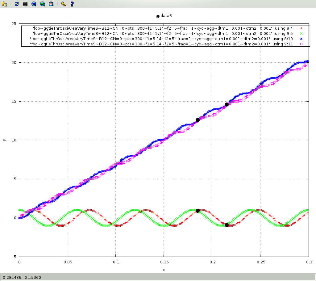
The following two figures show some of the beat occurences. In the first figure, the abscissa axis represents the number of points.
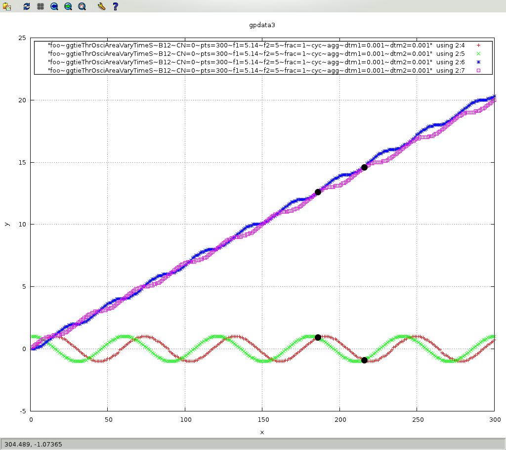
In the second figure, the abscissa axis represents the time, going from 0 to 0.3 second. This is considering the period is for 1 millis, or 0.001 second, then to complete the three periods (with 100 points per period) that would be 300*0.0001 or 0.3 second.The points of intersection where the beats occured are marked with large black points.