ASPL User Guide v 1.00
© 2025 Bassem W. Jamaleddine
21. 9Tying to Oscillators Over Time Asynchonously with Actual Time
Tying to Oscillators Over Time Asynchonously with Actual Time
ELEMENTS-GROUPING-CLASS: TIE_OSCILLATORS_AREA_VARY_TIME_ATIME_GROUP
Sample Workspace: TIEDOSCI_SYSTIMED
Script To Locate Beats : foo.pl
GG-function: ggthreadedtimedoscillatorS()
Get the oscillating waves asynchronously along their summed areas:
TP12 = ggthreadedtimedoscillatorS( .. ) where TP12 is a set variable
Tying to Oscillators Over Time Asynchonously with Actual Time
In context of tied attributes, think of ASPL programming as being a containment programming and variables that are defined within egC-feeder Udev can be aggregated and persisted during the runtime of the egC-Container. More specifically, the tied attributes data may be transitioned between the invocations of GG-function for the lifetime of the tied-session.
When ASPL is started with a specific namedspace that has tied attributes, the egC-feeder module is also loaded, and the lifetime of its lexical variables defined within ASPL's tied containment modules are persisted for the duration of the module-runtime (as long as the egC-Container is not being reloaded asynchronously by threading procedures).
However, if the tied class is being loaded asynchronously by threading procedures then the lexical variables are being reset (simply because the variables will live within the block of the code loaded by the thread, and their values cannot be maintained across subsequent calls of renewed threads, even if the thread has the same name).
We will avoid sharing variables between the threads (to avoid locking on these variables which will cause delay as the asynchronous threads will appear running in parallel while in reality they are running serially - this will effectively impact the temporal time when sourcing the tied functions).
One solution to run the threads asynchronously, is run each thread without having any common variable variable updated (in the same time) by another thread, and later stitch the variables after all asynchronously invocations. To understand this, consider the following example, where the the GG-function ggthreadedtimedoscillatorS() calls Udev's stitchLexicalScoped.
In this example, we demonstrate how asynchronously calls to the threading procedures are subsequently stitched. This is the fastest way to have simulation of two oscillators with actual time recorded on the system.
Get the oscillators for 100 points in 1 second, delay between two points is 0.01 for both oscillators:# aspl -wsname TIEDOSCI_SYSTIMED -groupingclass TIE_OSCILLATORS_AREA_VARY_TIME_ATIME_GROUP
① aspl>
TP12 = ggthreadedtimedoscillatorS(tiesess,TP12,points,100,frequency1,1,frequency2,1,roundfrac,1,aggregate,1,resetcycle,0,delay1,0.01,delay2,0.01)
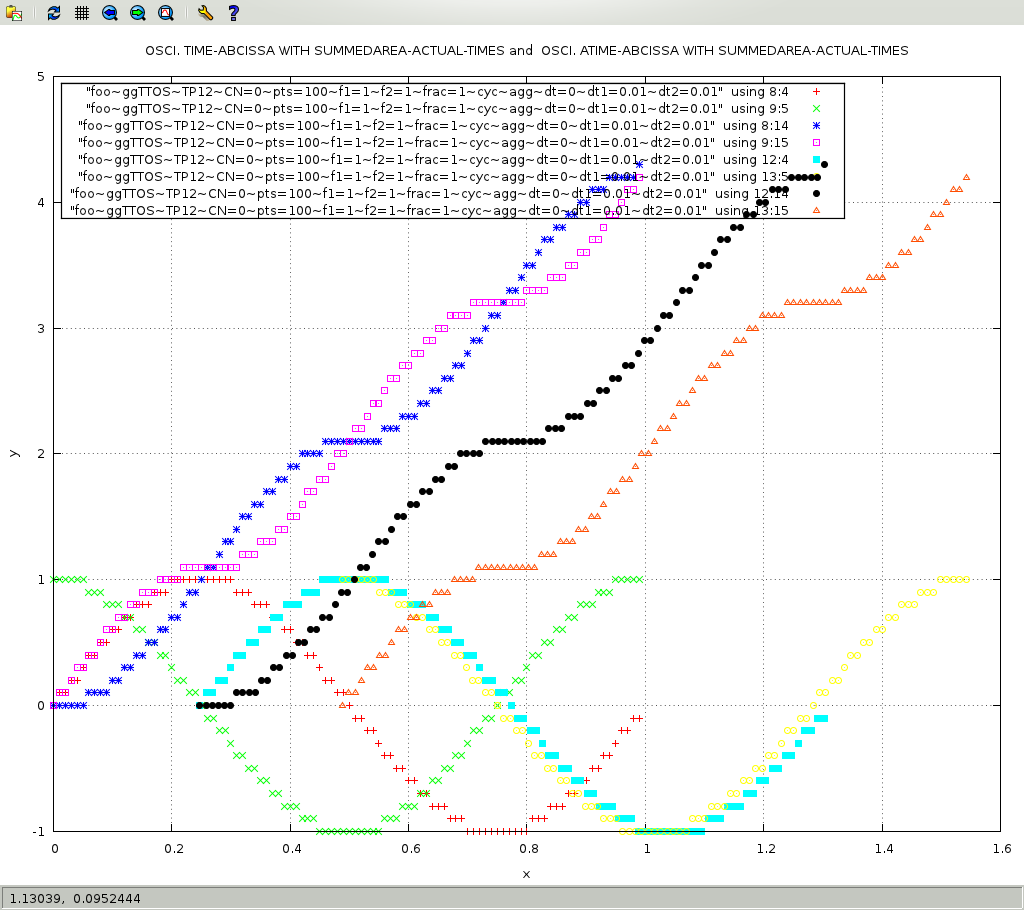
The following figure shows the two oscillators, each being sampled over theoretical time and actual time, along their summed areas. The actual time is the time gathered from the system clock, which is different than the theoretical time, since it will account for processing delays. The curve in yellow is the first oscillator started within the first thread, and the curve in light blue is the second oscillator started within the second thread. Even though both threads have been run asynchronously, notice the tiny delay between their actual startup times. The first oscillator actual time started somewhere between 0.2 and 0.3 second, and ended around 1.3 second, while the second oscillator actual time started around 0.5 second, and ended around 1.6 second. Of course their summed areas, shown in black-circles for the first oscillator, and red-triangle for the second oscillator, have also been shifted and didn't not intersect. If we allowed longer lapsed time for the one hundred sampled points, the actual processing time will have less impact (as the error in processing time dissipate) and the summed areas may intersect.
In theory, the first oscillator is the one shown in red-plus sign, and the second oscillator is the one shown in green-cross sign.
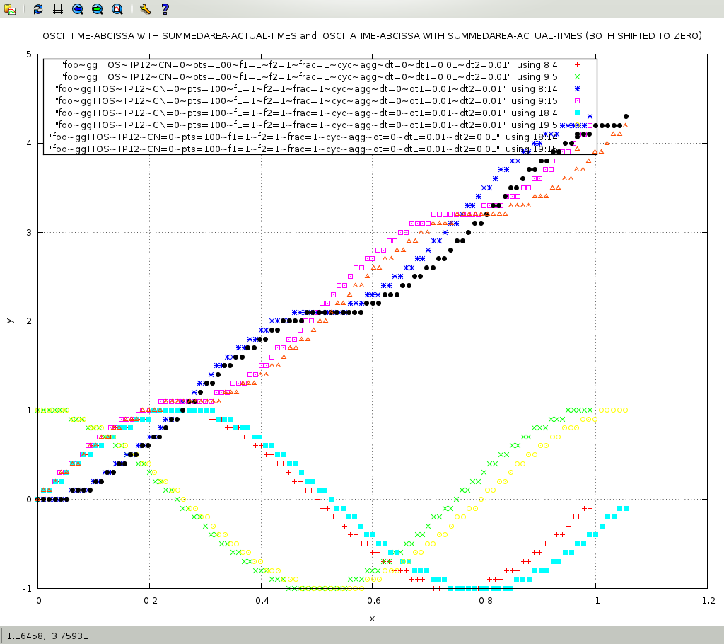
The following figure is for the same two oscillators discussed in the previous figure, however, the curves have been shifted so they all start at zero.
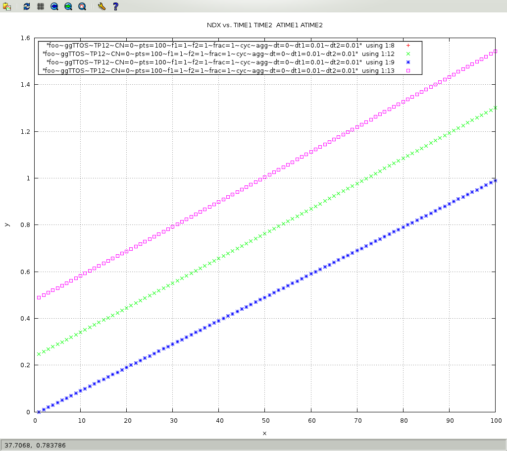
The following figure shows the index of the one hundred points on the X axis versus the time of the oscillating functions. TIME1 and TIME2 are for physical time and are shown in the red-plus and blue-asterik respectively: the mapping of 100 points vs. the 1 second total time, both lines are superimposed. ATIME1, actual time for the first oschillator, tooks approximately 1.3 second, and is shown in green-cross, ATIME2, actual time for the second oschillator, tooks approximately 1.5 second, and is shown in magenta-dotted-square.